Implicit Neural representations using sinusoidal activation

Audio compression

The reason we use the sine function as an activation function is because it is infinitely differentiable where as for a function like relu, the double derivative becomes zero. Let’s try regenerating an audio file by mapping coordinates in the grid with amplitudes

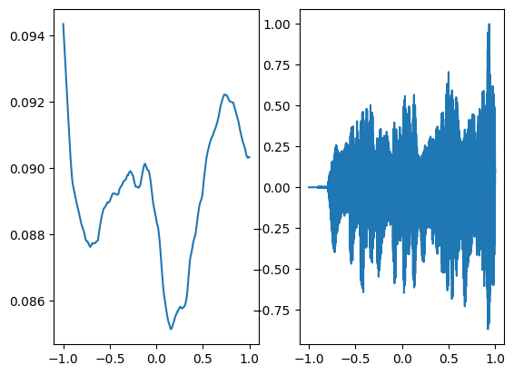
The following is the ground truth audio

We are using a neural network with 3 hidden layers and each layer consisting of 256 neurons and we are using mean squared error loss function and optimizing it using Adam with a learning rate of 0.0001. We are training the neural network for a total of 1000 steps and displaying every 100th result. As can be seen in the following figures as the number of steps increases both the graphs converge.

Description of neural network

Siren(
  (net): Sequential(
    (0): SineLayer(
      (linear): Linear(in_features=1, out_features=256, bias=True)
    )
    (1): SineLayer(
      (linear): Linear(in_features=256, out_features=256, bias=True)
    )
    (2): SineLayer(
      (linear): Linear(in_features=256, out_features=256, bias=True)
    )
    (3): SineLayer(
      (linear): Linear(in_features=256, out_features=256, bias=True)
    )
    (4): Linear(in_features=256, out_features=1, bias=True)
  )
)

Step 0, Total loss 0.025424
Step 100, Total loss 0.002972
Step 200, Total loss 0.001123
Step 300, Total loss 0.000861
Step 400, Total loss 0.000702
Step 500, Total loss 0.000586
Step 600, Total loss 0.000535
Step 700, Total loss 0.000538
Step 800, Total loss 0.000665
Step 900, Total loss 0.000362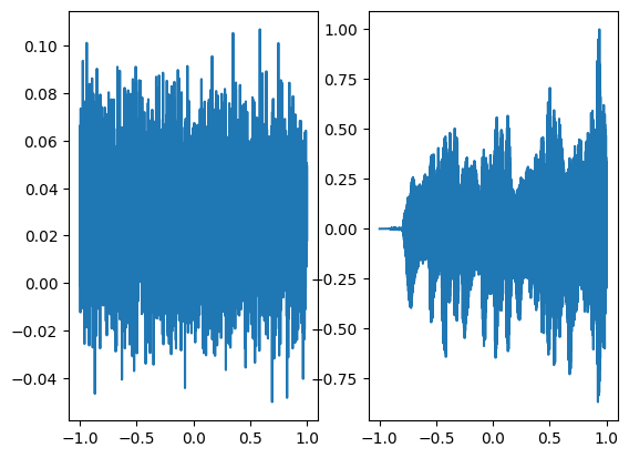

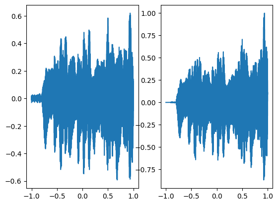
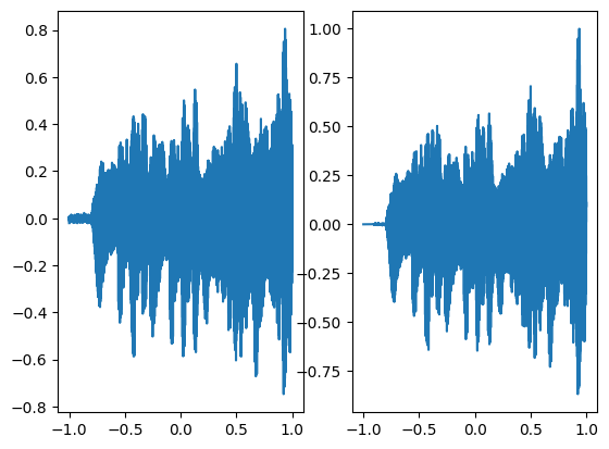
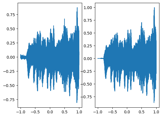
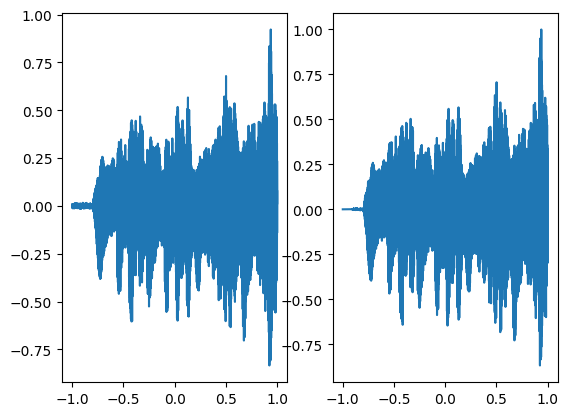
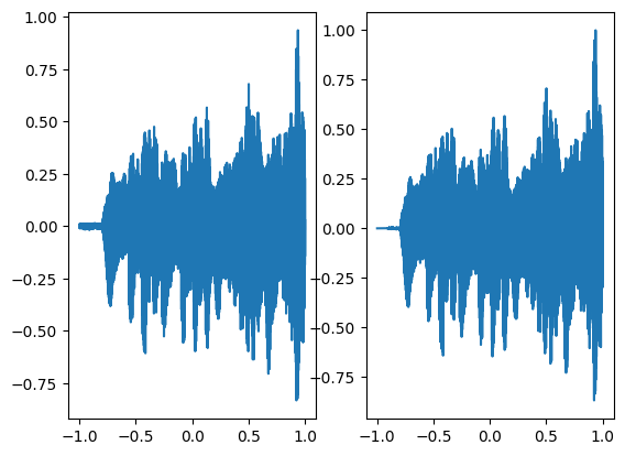
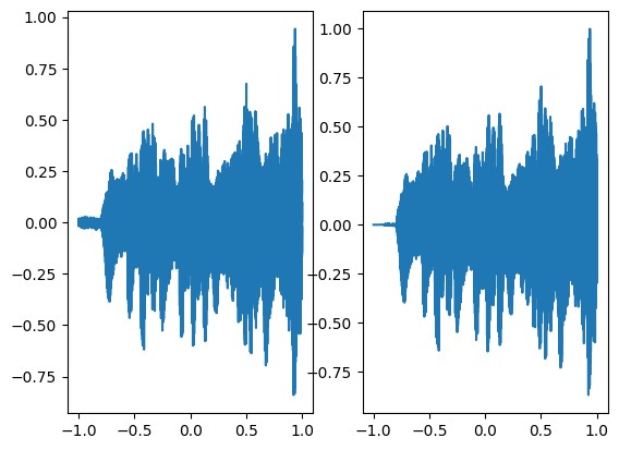
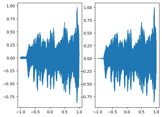
In the above graph the coordinates of the grid are squeezed to a single dimension (x-axis) and the corresponding model output is shown on the y-axis.

Following is the audio regenerated using a neural network with sinusoidal activation

There is a little bit of noise in the above regenerated audio signal but overall has a good performance

Let’s try using a different activation function such as relu and how well it can perform to regenerate audio and compare it with sinusoidal activation

Step 0, Total loss 0.032153
Step 100, Total loss 0.032153
Step 200, Total loss 0.032153
Step 300, Total loss 0.032153
Step 400, Total loss 0.032153
Step 500, Total loss 0.032153
Step 600, Total loss 0.032153
Step 700, Total loss 0.032153
Step 800, Total loss 0.032153
Step 900, Total loss 0.032153

Following is the audio regenerated through relu activation which is not at all close to the ground truth

How much memory do we save through this compression technique?

Memory of audio file: 1232886 bytes

Number of parameters in the neural network are 198145

Memory consumed by the neural network is 796343 bytes

Hence, we can conclude that passing the network parameters instead of the audio file itself can save space.

Image compression

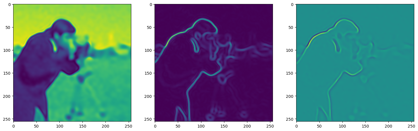
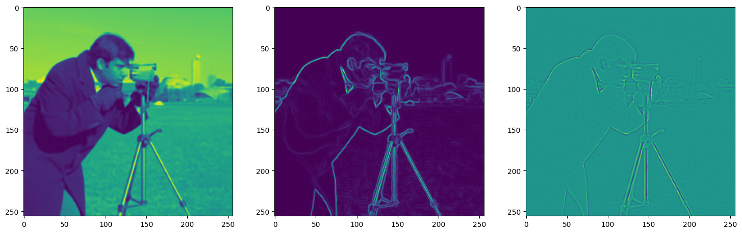
For the sake of an example let’s take the classic cameraman photo

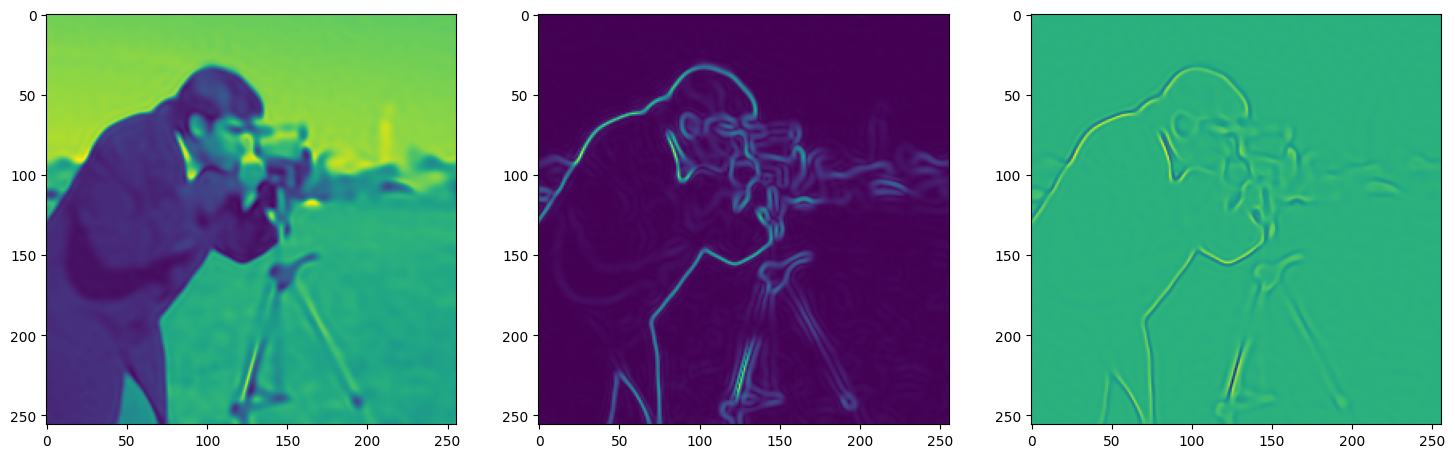
This is the architecture used for modelling the image, it contains 3 hidden layers and 256 neurons in each layer using the adam optimizer with learning rate 1e-4.

Siren(
  (net): Sequential(
    (0): SineLayer(
      (linear): Linear(in_features=2, out_features=256, bias=True)
    )
    (1): SineLayer(
      (linear): Linear(in_features=256, out_features=256, bias=True)
    )
    (2): SineLayer(
      (linear): Linear(in_features=256, out_features=256, bias=True)
    )
    (3): SineLayer(
      (linear): Linear(in_features=256, out_features=256, bias=True)
    )
    (4): Linear(in_features=256, out_features=1, bias=True)
  )
)

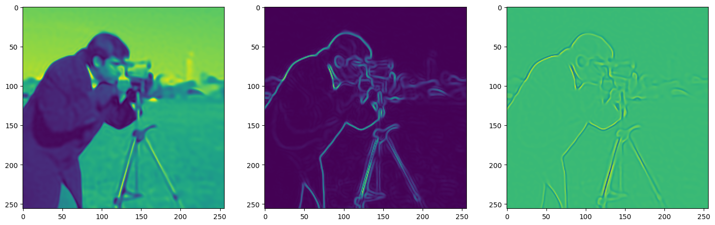
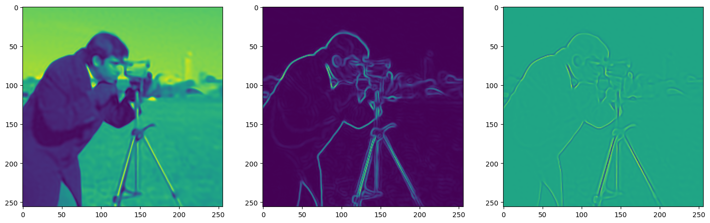
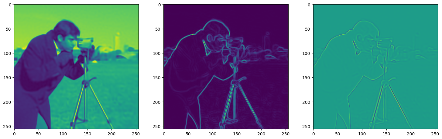
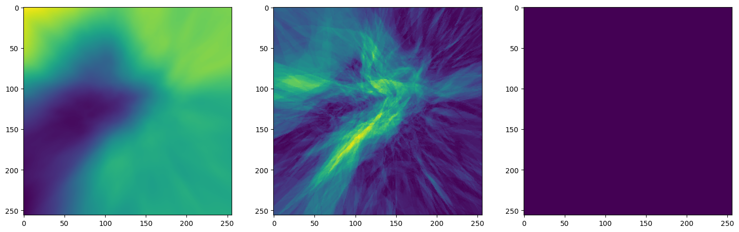
Now let us train SIREN model on our dataset i.e the image. The loss and the current state of the Network is displayed for every 50th element.

Step 0, Total loss 0.325293
Step 50, Total loss 0.012300
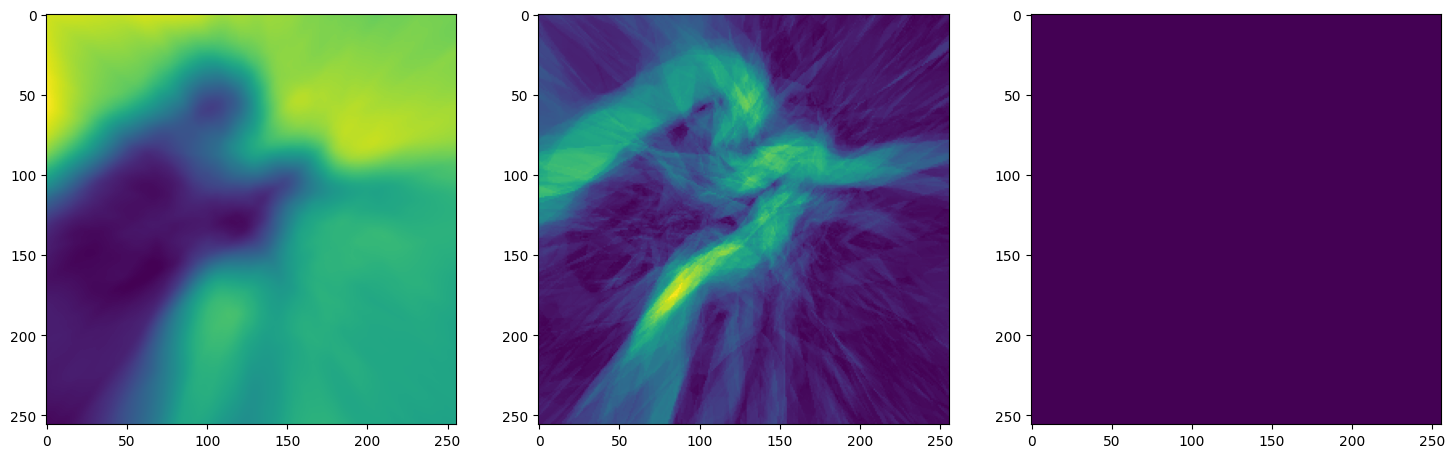
Step 100, Total loss 0.008443
Step 150, Total loss 0.006012
Step 200, Total loss 0.004077
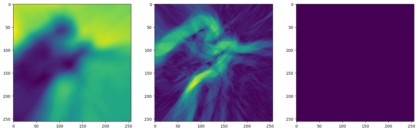
Step 250, Total loss 0.002673
Step 300, Total loss 0.001977
Step 350, Total loss 0.001566
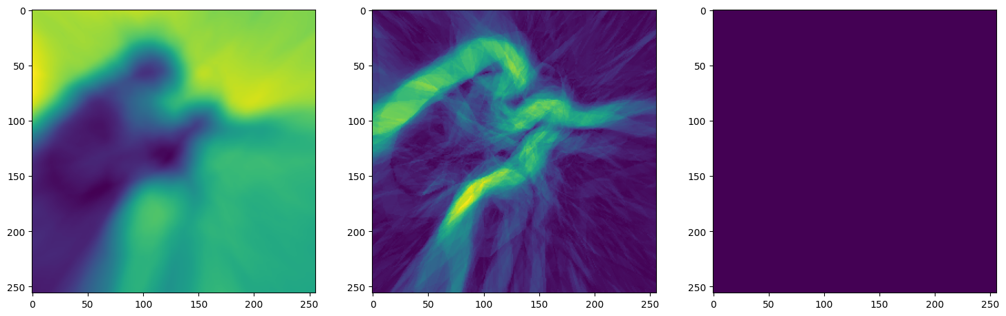
Step 400, Total loss 0.001294
Step 450, Total loss 0.001094
Step 500, Total loss 0.000939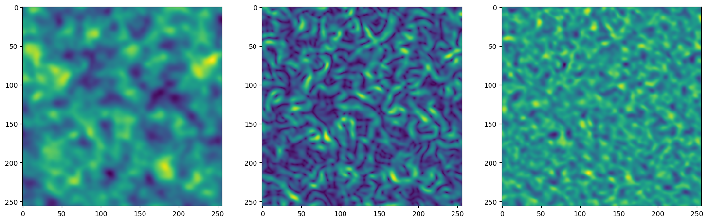

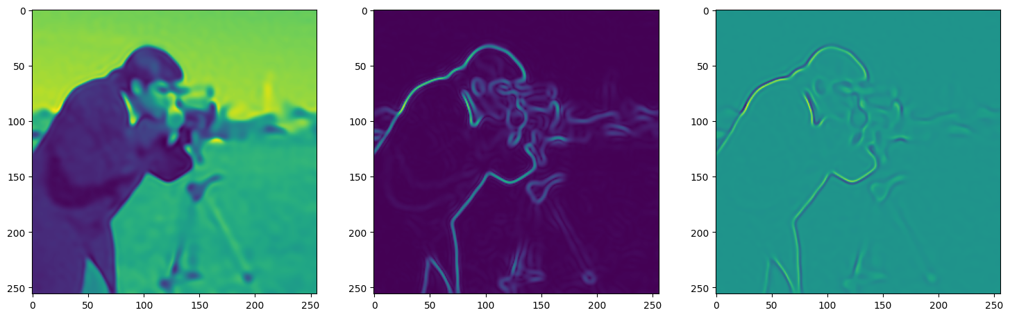
Let’s see how ReLU works in this setting. This is the architecture for the Neural Network:

Network(
  (net): Sequential(
    (0): ReLULayer(
      (linear): Linear(in_features=2, out_features=256, bias=True)
    )
    (1): ReLULayer(
      (linear): Linear(in_features=256, out_features=256, bias=True)
    )
    (2): ReLULayer(
      (linear): Linear(in_features=256, out_features=256, bias=True)
    )
    (3): ReLULayer(
      (linear): Linear(in_features=256, out_features=256, bias=True)
    )
    (4): Linear(in_features=256, out_features=1, bias=True)
  )
)

Step 0, Total loss 0.733969
Step 50, Total loss 0.077224
Step 100, Total loss 0.064925
Step 150, Total loss 0.057928
Step 200, Total loss 0.052542
Step 250, Total loss 0.048083
Step 300, Total loss 0.044299
Step 350, Total loss 0.041403
Step 400, Total loss 0.039117
Step 450, Total loss 0.037259
Step 500, Total loss 0.035712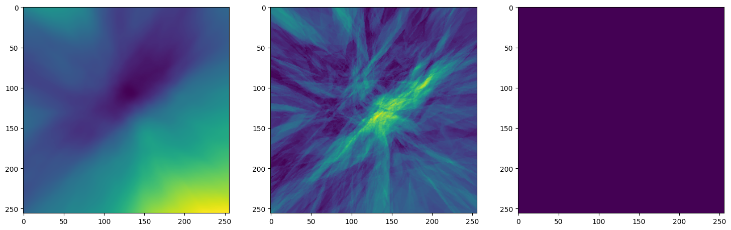

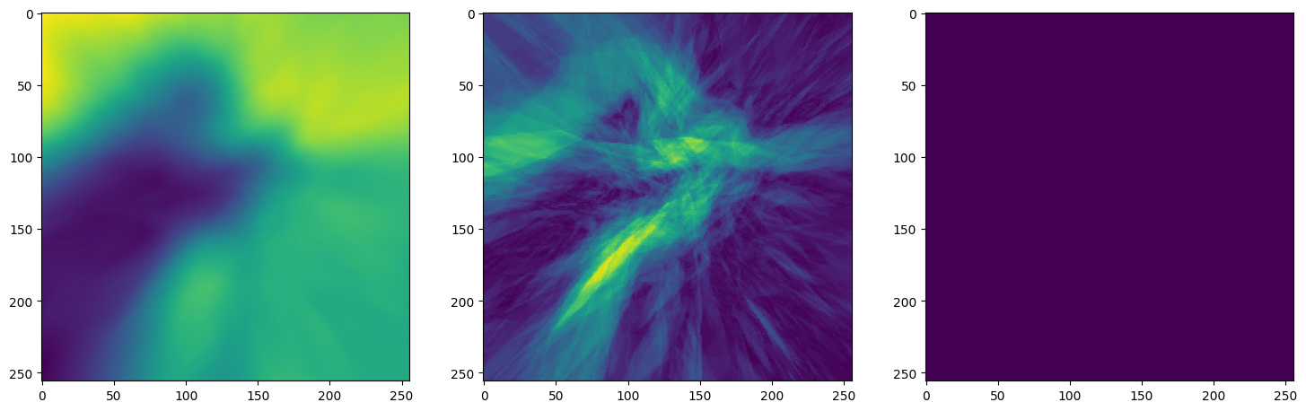
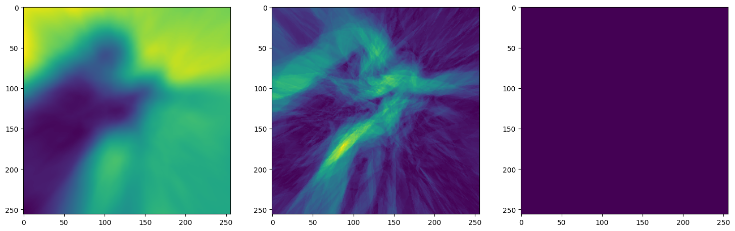
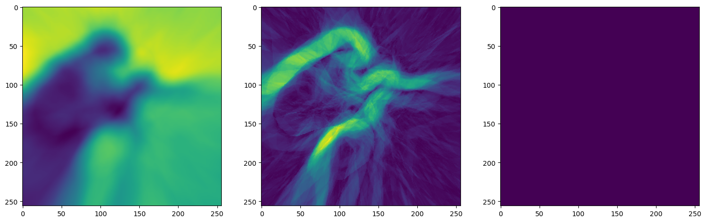
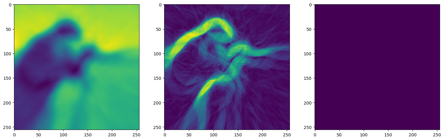
Note that the laplacian of the image generated by ReLU activation is constant (or you can say zero) because the second derivative of the ReLU function is zero, because it is a linear function. Hence, it does not perform well for transmitting signals.

Another takeaway for us was that the task of these kinds of Neural nets is to actually overfit over the data. By overfitting the data, it basically memorised the outputs for the given inputs. In generic Machine learning applications sinusoidal activation functions would not work at all.

This method is approximately 12 times better than the regular way of transmitting images. But the catch is that training the neural network for a single image of decent quality takes an hour on fairly strong computers. This renders this message of compression very unpractical. Hence, it is not used for real world data compression yet. If somehow the time required for training could be lowered, it would be quite usable in real life applications.