Mutual Information

Mutual Information

Mutual information is a feature utility metric that is used to measure associations between a feature and a target. It helps in finding out the features on which the target is most dependent on. Hence, we can narrow down the set of features/parameters we want to use to train a model reducing the training cost. Mutual information is similar to correlaton as it measures the relationship between two quantities. The advantage of mutual information is that it can detect any kind of relationship while correlation only detects linear relationships.

Mutual information derives relationships based on uncertainty. The mutual information (MI) between two quantities is a measure of the extent to which knowledge of one quantity reduces the uncertainty about the other.

Calculating mutual information for discrete random variables

If we denote mutual information by MI,

\[ \text{MI}=\hspace{0.1cm} \sum_{x,y} p(\text x,\text y)\log(\frac{p(\text x,\text y)}{p(\text x)p(\text y)}), \quad \text{where } p(\text x,\text y) \text{ is the joint probability of occurance of x and y and, } p(\text x) \text{ is the marginal probability of x.} \]

Clearly from the above formula we can see that if \(\text{x}\) and \(\text{y}\) are independent events, the joint probability of \(\text{x}\) and \(\text{y}\) \(p(\text x,\text y)=\hspace{0.1cm}p(\text x)p(\text y)\) and hence \(\text{MI}=0\).

Code

import numpy as np

def joint_prob(val_x,val_y,X,Y):
    n = len(X)
    count=0
    for i in range(n):
        if (X[i]==val_x and Y[i]==val_y):
            count+=1
    return count/n


def mutual_info(X,Y):
    n = len(X)
    unique_x = list(set(X))
    unique_y = list(set(Y))
    prob_x = [X.count(x)/n for x in unique_x]
    prob_y = [Y.count(y)/n for y in unique_y]
    MI=0
    for i in range(len(unique_x)):
        for j in range(len(unique_y)):
            px = prob_x[i]
            py = prob_y[j]
            jointp = joint_prob(unique_x[i],unique_y[j],X,Y)
            if jointp==0:
                continue
            else:
                MI += jointp * np.log(jointp/(px*py))

    return MI


X = ["A","B","C","A","B","C"]
Y = ["A","B","C","A","B","C"]
Z = ["A","A","A","A","A","A"]
W = ["A","A","C","A","A","C"]
print(f"Mutual information of X and Y is {mutual_info(X,Y)}") 
print(f"Mutual information of X and W is {mutual_info(X,W)}")
print(f"Mutual information of X and Z is {mutual_info(X,Z)}") 

Mutual information of X and Y is 1.0986122886681096
Mutual information of X and W is 0.6365141682948128
Mutual information of X and Z is 0.0

let’s veify our Mutual information score using the pre-defined function in sklearn.metrics

Code

from sklearn.metrics import mutual_info_score as MIS
print(f"Mutual information of X and Y through sklearn is {MIS(X,Y)}") 
print(f"Mutual information of X and W through sklearn is {MIS(X,W)}") 
print(f"Mutual information of X and Z through sklearn is {MIS(X,Z)}") 

Mutual information of X and Y through sklearn is 1.0986122886681096
Mutual information of X and W through sklearn is 0.636514168294813
Mutual information of X and Z through sklearn is 0.0

No matter what the value in X, the value in Z is always “A”, hence the two are independent and their mutual information score is 0.

Calculating mutual information for continuous random variables

Here, by continuous random variables we are assuming that random variables are continuous if they take values having float data type. For continuous random variables, the value of MI is given as follows.

\[ \text{MI(x,y)}=\hspace{0.1cm} \int_x \int_y p(\text x,\text y)\log(\frac{p(\text x,\text y)}{p(\text x)p(\text y)})dy\hspace{0.1cm}dx \]

Here, \(p(\text x,\text y)\) is the joint-probability distribution function of x and y, and \(p(\text x)\) is the marginal probability distribution function of x.

We may not always know the probability distribution of the data or the continuous random variables. Mutual information is also calculated as follows:

\[ \text{MI(x,y)}=\hspace{0.1cm} \text{H(x)}+\text{H(y)}-\text{H(x,y)},\quad \text{where H(x) is the entropy of x and H(x,y) is the joint entropy of x and y.} \]

In this method, we discretize the continuous random variables with the help of bins. The number of bins to be used to discretize the random variable is a parameter.

Let’s better understand calculting the mutual information score of continuos random variables through an example. In the following code, we have taken a continuous random variable following the normal distribution (X), a random variable with all zero values (Y), a random variable Z such that Z = 2x, and finally a uniform random variable W.

Code

def entropy(X,bins):

    binned = np.histogram(X,bins)[0]
    prob = binned / np.sum(binned)
    prob = prob[np.nonzero(prob)]
    entropy = - np.sum(prob* np.log2(prob))
    return(entropy)




def joint_entropy(X,Y,bins):
    
    binned_dist = np.histogram2d(X,Y,bins)[0]
    probs = binned_dist / np.sum(binned_dist)
    probs = probs[np.nonzero(probs)]
    joint_entropy = - np.sum(probs* np.log2(probs))
    return(joint_entropy)




def mutual_info(X,Y,bins):

    H_X = entropy(X,bins)
    H_Y = entropy(Y,bins)
    H_XY = joint_entropy(X,Y,bins)
    MI = H_X + H_Y - H_XY
    return(MI)

np.random.seed(12)
X = np.random.normal(0,1,30)
Y = np.zeros(30)
Z = X*2
W = np.linspace(1,10,30)

print("Taking number of bins as 10")
print("Mutual information of X and Y is: ",mutual_info(X,Y,10))
print("Mutual information of X and Z is: ",mutual_info(X,Z,10))
print("Mutual information of X and W is: ",mutual_info(X,W,10))

Taking number of bins as 10
Mutual information of X and Y is:  0.0
Mutual information of X and Z is:  2.8859175795054957
Mutual information of X and W is:  1.6342884121176722

The mutual Information between X and Y is 0 as Y is the zero vector. X is most dependent with Z as expected. One of the limitations of this method is to choose the number of bins but keeping the number of bins same for different features will maintain consistency.

Estimating mutual information using sklearn

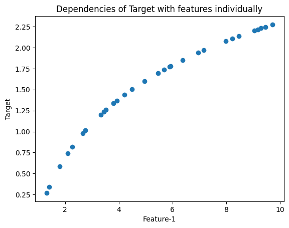
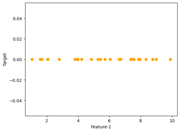
Let’s take an example where the target vector (W) is given by:

\[ \text{W}=\hspace{0.1cm}\alpha\log(\text x) + \beta \text{y}^2 \]

Here, \(\alpha\) and \(\beta\) are parameters. \(\text{x and y}\) are continuous random variables following uniform distribution.

Code

import numpy as np
import matplotlib.pyplot as plt

np.random.seed(42)
noise = np.random.normal(0,1,30)

alpha = int(input("alpha: "))
beta  = int(input("beta : "))

x = np.random.uniform(1,10,30)
y = np.random.uniform(1,10,30)
X = alpha*(np.log(x))
Y = beta*(y**2 )
W = X+Y+noise 

plt.scatter(x, X, label='alog(x)')
plt.title("Dependencies of Target with features individually")
plt.xlabel("Feature-1")
plt.ylabel("Target")
plt.show()

plt.scatter(y, Y, label='by^0.5', color='orange')
plt.xlabel("Feature-2")
plt.ylabel("Target")
plt.show()

alpha:  1
beta :  0

Code

from sklearn.feature_selection import mutual_info_regression as MIR
print(f"MI score of W and x is {MIR(X.reshape(-1,1),W)[0]}")
print(f"MI score of W and y is {MIR(Y.reshape(-1,1),W)[0]}")

MI score of W and x is 0.1342259837428359
MI score of W and y is 0